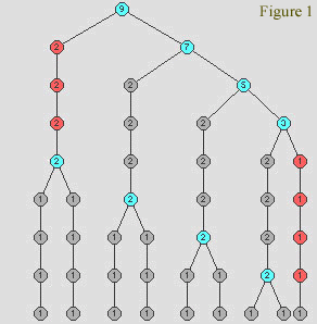
Figure 1:Time trees representation of a chord.
UFPr Arts Department
Electronic Musicological Review
Vol. 6 / March 2001
EMR Home - Home - Editorial - Articles - Past Issues
TIME TREES AS VIRTUAL WORLDS
Music can be described as data structures living inside its smaller particles, where time and space are combined into a single piece of information representing a sort of genetic code, the interpretation of which shows the existence of some cues for explaining and building music itself. Musical events can be read from these well-formed data structures also known as time trees, which are revealed if the interval is investigated by a model able to preserve all the significant information present in the corresponding physical phenomenon. The common sense model of the interval using only two whole numbers is not enough, for there is mathematical and acoustical evidence showing that the interval is an object possessing three different states which depend not only on the frequency but also on the intensity ratio. Entire spectral charts after being computed by time trees are converted into 3D virtual worlds from the processing of acoustical, geometrical, luminous and kinematic values, all of them related to the internal physics of the intervals. The visitors of such worlds can experiment real-time musical compositions while navegating and interacting with the sonic objects there defined [1].
To model music from the time and space structures computed in its lesser parts is quite different from mapping an arbitrary physical phenomenon into musical values. Whereas in the second case it is very hard if not impossible at all to find an evidence that its resulting sounds will be processed by the brain as music, a legitimate musical semantics is supported in the first case due to the basic perception laws of two-frequency stimuli and to everything the intervals represent in building and understanding music. Besides, further formal handling with the intervalic phenomenon shows more than only music inside the intervals. These time and space structures, known as time trees [3, 7], when converted into virtual worlds are naturally associated to information groups corresponding to acoustical, geometric, luminous, and kinematic values all of them calculated in the physics of the inner world of the intervals (Figure 1). The virtual worlds so defined are 3D environments which are capable of detecting the presence of visitors and giving them means for the experimentation of immersion, interaction, and navigation through their objects which have shape, color, musical and kinematic behaviours. In this way, the visitors can do real time compositional voyages and image synthesis while walking the world and touching the objects there defined.
Figure 1:Time trees representation of a chord.
Time trees are suitable for virtual worlds just because they have all the constituents for that. Indeed, they carry sonic objects having a hierarchy of times and places at well defined positions in the 3D space, each of them having a form, a colour, and a musical behavior from which it is possible to build a program for generating intervalar virtual worlds, that is, a multimedia program capable of simulating the physics of the interval as well as providing some important tools to the visitor for interacting and navigating in the virtual world. The immersion will help the visitor in the process of feeling himself or herself as a legitimate part of the interval's internal reality. The interaction means the ability to drive the existing musical behaviours inside the sonic objects, and the navigation means the ability to translate himself or herself through the virtual world in any direction, at any velocity, and, in general, looking for being next to a given sound group that exists at a given place of the space and time. As the nodes besides being placed at well defined positions are associated to moments and durations, a voyage through an intervalar world may also have the meaning of a time voyage as well. The time flow defined by the chronological sequence of the composition can be changed according to the navigation decided by the visitor, who in this way will create a new composition that will reflect the route done by himself or herself.
Every node in a time tree, as the primordial of a Major-Sixth at the low state in Figure1, becomes alive at a given time and will stay alive for a duration which is a nuclear information of the node itself. This information is also related to the topology of the tree so that when a node is taken into account all its descendent nodes are automatically taken into account as well. Being this a central conception in the computation of instruments, the resulting timbre at each moment will be affected by the topology at the corresponding tree region.
The musical behaviour of a given node is the emission of a group of sounds which is computed from the kinematic state of the intervalar object at the node. This situation brings about the concept of orthogonal note (see definition below) whose computation at a node P is done by using the measuring-SHM method[3] which extracts from the intervalar object a CM (circular and uniform motion) having a tangential velocity equal to the projection Vxz of the velocity V (at the a node P) on the xz plane; and extracts another CM corresponding to the Vyz projection of the velocity V on the yz plane. The simple harmonic motion associated to each CM, that is, the motion executed by the projection of the point executing the circular motion on a straight line crossing its center is the so-called measuring-SHM, being both harmonic motions taken on the z-axis:
xz(t) = Axz sin(2pFxz.t + fxz)
yz(t) = Ayz sin(2pFyz.t + fyz)
As there are two simple harmonic motions at each node, there is enough information about two simultaneous musical notes. An orthogonal note is just this couple of notes, one for each of the xz e yz projection planes [2].
The calculation of the amplitude is straightforward if compared to the initial phase angle and the frequency, for the measuring-MHS method is just the radius of the circunscribed circular motion. By just taking the components of vector P in the xz and yz planes, the amplitudes are respectively:
Axz= (Px² + Pz²)1/2
Ayz= (Py² + Pz²)1/2
On the xz plane, the measuring-SHM is the motion defined by the projection of Pxz , which is the projection of P on the xz plane on the z-axis. The value of the initial phase angle will depend basically on the angle yP, which is the angle between the vector Pxz and the z-axis, and on the orientation of the velocity vector Vxz- Pxz. Moreover, for determining the direction of the rotation it will be necessary the handling of yV, which is the angle between the vector Vxz and the z-axis. After obtaining the direction of rotation, the initial phase angle of the measuring-SHM is calculated from yP and by taking into account the existence of a p /2 shift between the angle yP and the phase angle f of the measuring-SHM. Therefore:
fxz= p /2 ± yxz
fyz= p /2 ± yyz
The plus sign indicates a counterclockwise rotation.
2.1.3. Frequency
The calculation of the frequency follows the basic scheme: F = w /2p; as w = |vT| /R, it follows that: F = |vT| / 2p R. That is, the calculation is done from the amplitude of the measuring-MHS (the radius R ) and from the tangential velocity vT [3]. The resulting values for the xy and yz planes are respectively:
Fxz = (1/2p ) [(Vx² + Vz²)/(Px² + Pz²)]1/2 . |sendxz|
Fyz = (1/2p ) [(Vy² + Vz²)/(Py² + Pz²)]1/2 . |sendyz|
Being d = |yP-yV|. From these equations, spectral contents and behaviour are assigned to each node as determined by the existence of a population of measuring simple harmonic motions defined by the descendent nodes. All the motions found in this way are grouped in a single additive synthesis instrument [5, 6].
According to the theory of time trees, every node will be alive at a given instant t that will last for d units of time in the sense that it will be associated to geometrical and sonic forms. If the interpretation of the sound may be said unique, the same is not true for the geometry, for there are more than one way of interpreting the reading of the form from the data found inside the node and from the topology of its subtree. This reading of the underlying geometry falls on the instrument architecture, on the envelopes, and on the rhythmic patterns inherited from the time trees. For instance, in the image of Figure 2 the shapes up to a certain level of detail are computed from informations living strictly inside the spectral chart. Another way of building the visual aspect of the object is to assign 3D shapes to the nodes by assuming a greater freedom in the correspondence between the intervalar phenomenon and the geometry. Further on, a program called (Cubismo) assigns regular and semi regular polyhedrons to the nodes. The main advantage in this case is to make possible a very fast computation of a geometry which is a basic requirement of virtual worlds made up with current technology [8, 9].
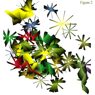
Figure 2: Shapes are computed from information taken from inside a spectral chart.
2.3. Color
The correspondence between notes and colours depends on the definition of a vector space (ROI) for representing the notes having the following features: (1) it preserves and expresses the basic aspects of pitch perception, as the segmentation of the audible frequency range in octaves, that is, the ability of recognizing a frequency and their power of two multiples as the same note, and (2) it adopts the intervalar loudness principle, a concept derived from the equilibrium theorem [1, 3], which is defined as follows: the intervalar loudness (A) of a spectral component, also called H-unit, is the product of the amplitude by the square frequency, that is:
A = af ²
Therefore, two H-units will be in equilibrium when the intervalar loudness is the same for both. In every spectral chart there are a minimal intervalar loudness (Amin = [af ²]min) and a maximal intervalar loudness (Amax = [af ²]max) in the midst of its population of H-units. These values are related in the following concept:
The intervalar loudness range (U) in a spectral chart is given by:
U = log (Amax/Amin)
In this way, any H-unit will fall inside this range, and a scale of intensity levels is defined that is ready to be mapped into levels of luminosity.
In the ROI space (Figure 3), the notes are organized so as to satisfy the correspondence criterion between light and sound at their respective perceptual spaces. A note [a, f] from a spectral chart having an intervalar loudness range of U will assume in this space the following coordinates (r, o, i), that is, ratio, octave, and intensity:
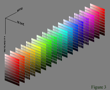
Figure 3: The organization of notes in the ROI space.
o = trunc(log 2 (f / fb))
r = f / (fb.2 o)
i = (1/U)log 10 (af ²/ [af ²]min)
Where fb is the lower limit of the audible frequency range. In order to proceed the calculation of the color associated to a H-unit it is necessary to adjust the limits of the corresponding values. As the octave o is a real value in the range 0..9; r is a ratio lesser than 2; and the intensity i is a real value in the range 0..1, a [r, o, i] component will correspond to the following color in the hsb system (hue, saturation, brightness):
h = 360 (r - 1)
s = o /10
b = i
Cubismo is a program written in Java 3D [10] for building virtual worlds enclosing all the above described calculations on form, color, and musical behaviour from a spectral chart. The first action of Cubismo's constructor method, which has a chart as an argument, is to build the superstructure of the scene graph as shown in Figure 4.
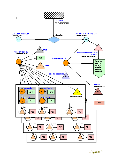
Figure 4: The process of building the superstructure of a scene. (Figure provided only in Portuguese)
SPECTRAL CHART SYNTAXnew Cubismo(chart);
The chart is initially computed by the time-tree expert program Carbono [4] in the SOM-A syntax, then it is converted by the program Ilusom [4] into a more appropriate form for Cubismo in the task of constructing a virtual world. The commands are as follows:
CARTA ntnt = number of additive notes in the chart
NOTA_ADITIVA n pop tzr dur ins1 ins2
n = order number of the timbre
pop = population of notes in the timbre
tzr = starting time (in seconds)
dur= duration (in seconds)
ins1 = yz-plane instrument
ins2 = xz-plane instrumentUNIDADE_H_0 can atq tec lsb msb p1 p2 p3 p4 orto
UNIDADE_H_1 can atq tec lsb msb p1 p2 p3 p4 ortocan = midi channel
atq = atack time
tec = midi key number
lsb = pitch bend lsb
msb = pitch bend msb
p1= signal weight at the sound source P1
p2= signal weight at the sound source P2
p3= signal weight at the sound source P3
p4= signal weight at the sound source P4
orto= plane of acoustical projection (upper=0 or frontal=1)
Geometrical commands:
posicao x y z (position of the node; in meters)
posicao_ascendente xa ya za (position of the ascendent node; in meters)
orientacao rx ry rz (orientation; in degrees)
tamanho w (size)
rgb r g b (0..1)
arvore i (tree number)
For the sake of ilustration, it follows a small section showing a single additive note having 3 spectral objects (6 H-units) from a chart of 322 additive notes.
CARTA 322 notas aditivas
;---
NOTA_ADITIVA 1 3 0 0.416 I92 I91
;---
UNIDADE_H_1 11 2 106 11 64 52 0 23 27 1
UNIDADE_H_0 10 3 105 22 50 82 0 23 1 0
posicao 1.33 1.281 1.429
orientacao 222.724 230.36 221.891
tamanho 11.598
rgb 0.531 0.386 0.371
posicao_ascendente 1.33 1.281 1.429
arvore 46
[fim_unidade_H]
;--------------------
UNIDADE_H_1 11 2 115 80 65 56 0 24 31 1
UNIDADE_H_0 10 2 115 66 60 80 0 23 0 0
posicao 1.273 1.334 1.429
orientacao 163.815 285.18 43.07
tamanho 3.547
rgb 0.840 0.530 0.157
posicao_ascendente 1.33 1.281 1.429
arvore 46
[fim_unidade_H]
;--------------------
UNIDADE_H_1 11 1 43 114 61 32 0 13 13 1
UNIDADE_H_0 10 1 65 25 75 61 1 16 0 0
posicao 1.31 1.258 1.311
orientacao 300.196 147.427 222.33
tamanho 6.431
rgb 0.530 0.821 0.220
posicao_ascendente 1.33 1.281 1.429
arvore 46
[fim_unidade_H]
;--------------------
[fim_nota_aditiva]
;--------------------
3.1. The Scene Graph Superstructure
The constructor method's first step is to define an object u from the SimpleUniverse class as the root of the virtual world.
u = new SimpleUniverse(c);
Then a Locale object is automatically created as the single descendent of u. This Locale will have two descendents: one on the left for holding all the world's sonic, luminous, and geometrical objects, composing the branch Light, Geometry, and Sound of the scene graph, and another on the right composing the branch Visualization and Navigation, for handling position, orientation and motion of the camera according to parameters extracted from the chart itself.
At the root of this left branch, it is defined a node called cena as an object from the BranchGroup class.
cena = ramoLuzGeometriaSom(c);
Its first descendant is the node transformaCENA, which is a TransformGroup object that will be ascendant of every sound and light object in the world u. Any change in transformaCENA will affect all the objects in the left branch. A ground (a Shape3D object) for helping spatial localization is included as a leaf descendant of transformaCENA. The building of this left branch follows strictly the interpretation of the chart by reading all additive notes from the first to the last one. At each note the program catches position and orientation of the ascendant node, position and orientation of the node itself, the colour of the node, sets up a sensibilization volume for collision detection (between note and camera), and prepares a Midi message to be sent later on to the sonic device. The musical parameters coming subsequently in the chart are used to create the note as an object associated to the node. The steps in the 3D geometrization of an orthogonal note are: (1) definition of a sensible region (boundingSphere), (2) translation to its [x y z] position, (3) rotations in x, y, and z-axis in order to be oriented according to the chart, (4) computation of the form, and (5) assignment of material properties. At the end of a group of H-units, or at the end of the command NOTAS_ADITIVAS, a geometrization of timbres must be done by considering the group of notes defined in the subtree, that is, the links joining descendant and ascendant nodes are drawn in the 3D space, as well as the painting of the triangular faces defined by a node and its descendants. All the building of this branch is joined to the universe u according to the line:
u.addBranchGraph(cena);
At the root for this right branch, is defined the node vista as an object of the class BranchGroup.
vista = ramoDeVista();
Besides its usual function in bringing the scene into view, the camera represents and embodies the visitor in his or her navigation through the world. In view of this fact, the camera must be animated, like any other object under the graph could be, in order to create the sensation of navigation in the visitor. In order to animate the camera, the program uses a powerful interpolator object from the class RotPathPositionInterpolator which will assure a complete visit to all objects in the world. The kinematic values for such an animation, that is, the right camera displacement, velocity, and orientation which are necessary to place the visitor next to the current sonic objects at the right time and have all of them inside its field of vision, are calculated from the times associated to the events in the spectral chart. When the interpolator object has the coordinates of all the nodes to be visited, the orientations for the camera everywhere, and the velocities in each one of these segments, it is able to imposes through the transform associated to the object a 3D animation to the camera according to the chart's natural tempo. Otherwise the program will consider the active interaction from the visitor. All the building of this branch is joined to the universe u according to the line:
u.addBranchGraph(vista);
4. Conclusion
Inside an intervalar world, such as the one shown in Figure 5, it is possible to compute proper sounds at any 3D coordinates,
and not only where the nodes are placed. The same coordinates inside another world will sound differently. Therefore,
besides the sound groups defined by the time tree nodes, other sounds can be generated from the visitor's position
and velocity. Here the visitor is taken as an aggregated moving node, able to see and hear how the world is and
able to introduce what he or she is doing in the world as he or she travels and touches the objects, as a guided compositional process. This is the meaning of the concepts of interaction, imersion and navigation, when the virtual world
is also a time tree.
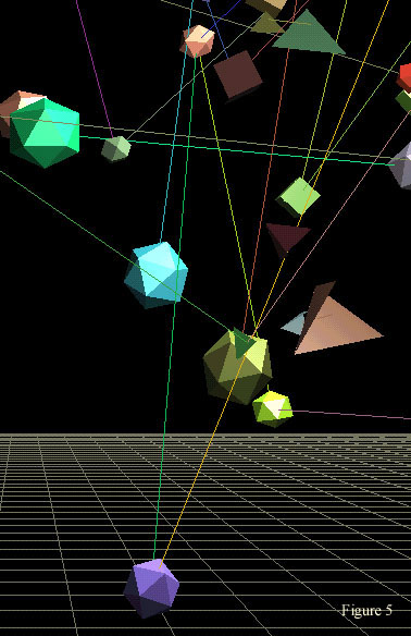
Figure 5: Wondering inside an intervalar world.
[1] Arcela, A., O objeto intervalar, On-line document: http://primordial.cic.unb.br/, Brasília, 1999.
[2] Arcela, A., Fundamentos de computação musical, VI Escola de Informática da Região Sul, Sociedade Brasileira de Computação (SBC), 1998.
[3] Arcela, A., As árvores de tempos, On-line publishing: http://primordial.cic.unb.br/, Brasília, 1996.
[4] Arcela, A., "Publicações/programas" , Laboratório de Computação Multimídia, On-line document: http://primordial.cic.unb.br/, Brasília, 1995.
[5] Arcela, A., "A linguagem SOM-A para síntese aditiva", Anais do I Simpósio Brasileiro de Computação e Música, Caxambu, Sociedade Brasileira de Computação (SBC), 1994.
[6] Miranda, E. R., Computer Sound Synthesis for the Electronic Musician, Focal Press, UK, 1998.
[7] Arcela, A., "Time-trees: the inner organization of intervals", Proceedings of the XII International Computer Music Conference, The Hague, International Computer Music Association (ICMA), 1986.
[8] Lévy, P., Cibercultura, Editora 34, Brazil, 1999.
[9] Negroponte, N., Vida Digital, Companhia das Letras, Brazil,1995.
[10]Sowizral, H. et. al., The Java 3D API Specification, Addison-Wesley, USA, 1998.
Aluizio Arcela, University of Brasilia, Department of Computer Science, Brasilia, Brazil.
email arcela@cic.unb.br